Conditional formatting

Even the best reports sometimes require that some information be emphasized in order to be more visible to the observer and help him to make certain conclusions. Conditional formatting is an Excel functionality that emphasizes the appearance of a particular cell or group of cells based on one or more rules. The appearance is formed on the basis of the data value or satisfaction of the conditions specified in the formula.

In order to apply conditional formatting, we first need to select the range of cells that we want to format. Most often it is a column in the report, but we can choose more columns at the discretion. Then, in the Home ribbon, by clicking the Conditional Formatting button, we’ll open a menu that offers many options for conditional formatting.

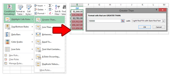
The first set of options is called Highlight Cell Rules, and it is used to emphasize a cell or group of cells that meet a certain requirement in relation to the value of the data. Under emphasis, it is usually assumed that they will be displayed in a different color of text and background in relation to other cells (eg, red text on a pink background), although it leaves the user the option to select the display format himself. And the conditions that can be set are: greater than the set value (Greater Than), less than the set value (Less Than), between two values ​​(Between), equal (Equal To). These conditions relate to when cell content is composed of numbers. If the content of the text is text, we will be able to specify the condition based on the text that the cell contains (Text That Contains); if the content is a date, we can provide a condition based on the date (Date Occurring). Also, there is an option to mark the Duplicate Values. After the start of each of these options, a dialog box will open in which we enter one or more parameters and choose the formatting style. After confirmation conditional formatting, based on the given criteria, takes place.

The second set of options is called Top/Bottom Rules and is used to conditionally format the smallest or largest cell values ​​from the selected set based on a given criterion. They offer options: Top Ten Intems, Top 10% , Bottom Ten Items, Bottom 10%, Above Average, Below Average. Unlike the last two options, the first four options offer the ability to parameterize the conditions. For example, we can formulate the first 3 cells by value, or cells that make up 20% of the total value of a given set. Formatting cells is easy and is done in a similar way to the first group of options for conditional formatting.

Then, 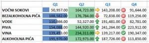there are three more groups of conditional format options: Data Bars, Color Scales, and Icon Sets. They differ from the first two groups in that they always refer to all the cells of the selected set. Data Bars options allow you to create mini-charts displayed for the selected cells in the form of a bar, which will appear in the background of each cell. For them, we can determine the color and fill style. The Color Scales group of options allows you to fill the background based on a given criterion, which indicates a growth or decrease in the value by the colors of the background. The Icons Sets group of options helps us to show trends in cell value changes using icons that will appear to the left of the value.

Each of the above groups of conditional formatting options has the More Rules option at the bottom. By selecting this option, you enter the menu in which parameters for conditional formatting can be specified in detail.