
Cat Icon Array Chart
I got an e-mail today from my wife who is a big cat lover. She says YouTube suggested her to watch the „Cat Icon Array Chart“ video. And since there is often a need to show the share of a value in a whole, using icon array chart, I decided to write a “recipe” that would teach you how to present data this way, without really using charts.
In cell A1 enter the number that represents the percentage that should be displayed. We need to change the font color in this cell to red. Then we will create a matrix of dimensions 10×10. In the column on the left, enter the numbers 0 to 9, and in the row above the numbers 1 to 10. We fill the matrix with the cat symbol that is obtained using the Webdings font and the appropriate code (use the Widows Character Map program to find the code).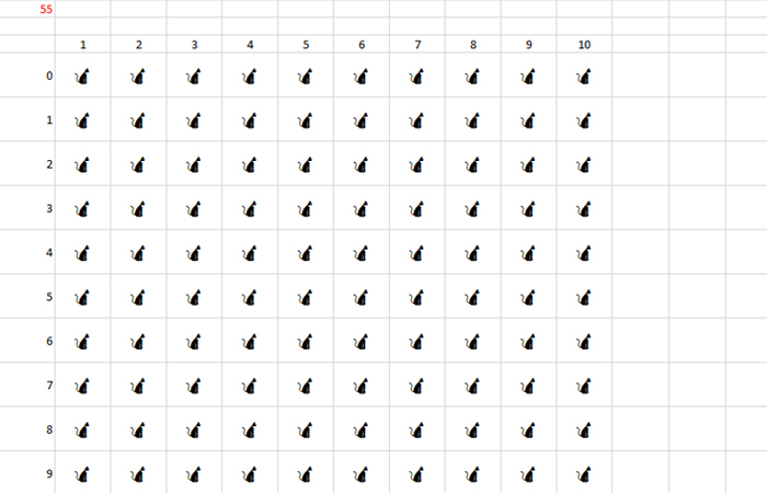
Then it is necessary to paint the background of the worksheet and the background of the matrix for better visual appearance. The numbers in the column to the left and the row above should be colored in the same color as the background of the worksheet, so they shouldn’t be visible.
Finally, we still need to select all the cells in the matrix and create the appropriate conditional formatting rule. In the Home tibbon open the Conditional Formatting menu, and then select New Rule. When the dialog box opens select the option to enter the formula and use the following expression:
$A$1>=(($A4*10)+B$3)
Then set that, if the condition is met, values in the cell are coloured dark red.
If you have done everything properly, all „kittens“ whose number is less than or equal to the one shown in cell A1 will be colored dark red. For example, if we entered number 55 we’ll have 55 dark red cats within a matrix. Changing the value of a cell A1 will also update the matrix, coloring more or less „kittens“.