Loan repayment
Financial functions in Excel allow for a variety of discounting operations. PMT function, for given present value, interest rate and number of periods calculates the total repayment value (annuity). How much, in this case, goes for the principal and how much for interest? To get answers to these questions you need to use the PPMT and IPMT functions.
The PPMT function has the following syntax:
PPMT(<rate>,<period>,<number of period>,<present value>,
[<future value>],[<type>])
The IPMT function has the same syntax:
IPMT(<rate>,<period>,<number of period>,<present value>,
[<future value>],[<type>])
The rate represents given interest rate, the period is the repayment period, and the number of periods indicates the current period for which the calculation is made. The present value is the initial value, and the future is the discounted value. The type of calculation can be 0, if the payment is made at the beginning, or 1 if it is done at the end of the accounting period.
Let’s see how this is used to calculate loan repayments! We will create a table with the following columns:
- YEAR
- LOAN VALUE
- PRINCIPAL REPAYMENT
- INTEREST REPAYMENT
- ANNUITY
- REMAINING VALUE
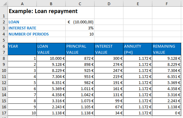
Above the table we will enter: LOAN (C2), INTEREST RATE (C3) and NUMBER OF PERIODS (C4). If we take a loan the field, where we record the value of the loan (present value), there must have a negative sign. If we would give a loan it would be a positive number. We will enter a value of -10000 in this field. The interest rate is 3% and the number of periods is 10.
The value of the principal is calculated using the following formula:
=PPMT($C$3,A8,$C$4,$C$2)
And we calculate the value of interest in this way:
=IPMT($C$3,A8,$C$4,$C$2)
Column A contains the number of periods for which the calculation is performed. By copying the formula it will be updated for the number of the current period. An annuity is the sum of interest and principal, and we can also calculate it using the formula:
=PMT($C$3,$C$4,$C$2)
The first row in the LOAN VALUE column is 10000, and each subsequent one is calculated using the formula:
= B8-C8
which is the value of the loan less the repaid principal. We see the remaining value in the column REMAINING VALUE. Here we use the same formula as in column B.
In this “recipe” you could see a simple way to calculate the loan repayment, in practice it is much more complicated and depends on the bank policy.