Parallel periods

The Power Pivot add-in allows you to make different calculations depending on the time period in which the sales occurred, by writing formulas in DAX language. To use these features you need to have one of the latest versions of Microsoft Office Pro Plus. Since many do not have this feature, it remains only to deal with the traditional lookup functions about which application I’ll write in following „recipe“.

The approach I will show you is more difficult than using formulas with DAX functions, but it allows you to calculate sales in parallel periods using functions that have long existed in Excel, and today also in many of its clones. So, if the management has “squeezed” you for a “more expensive” version of the Office package, and asks you for complex reports, here are ideas on how to answer the challenge.

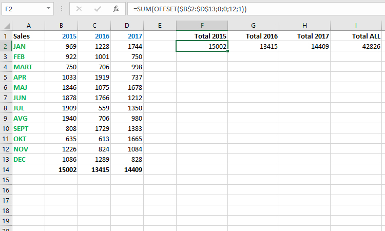
As an example we use the table which contains sales data, shown in rows by month, and in columns the sales per year for a period of three years. Total turnover by years can be calculated by summing the corresponding columns, and we can also use the OFFSET function where as an argument we give the whole table, and then we specify which column to summarize. This function is an argument of the SUM function, and the summation formula by years is:

=SUM(OFFSET($B$2:$D$13;0;0;12;1))

Depending on the year we would change the parameters that indicate which column is being aggregated. The OFFSET function also allows multiple columns to be summed, so if we want to calculate the turnover for all three years we will write the formula:

=SUM(OFFSET($B$2:$D$13;0;0;12;3))

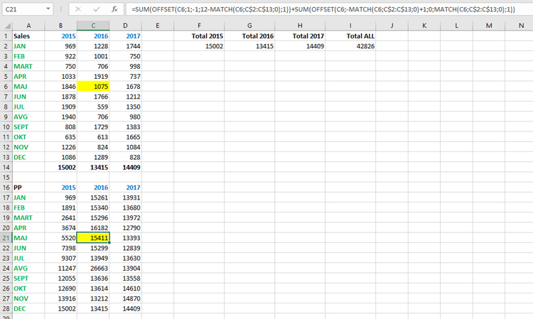
Often there is a need to calculate the sum of sales in the previous year, in relation to the given month, which is sometimes called the “parallel period”. Such a calculation is the sum of operations in the previous year, from the given month to the end of the year, as well as in the current year, from the beginning to the given month. How is this calculated?

Let’s create a formula beginning with some value in the middle of the year, say for May 2016. To find the index of array in which the value for May is located we can use the formula:

MATCH(C6;$C$2:C$13;0)

It will calculate that given cell is 5th element of a C column, which has total count of 12 elements. Formula:

=SUM(OFFSET(C6;1;-1;12-MATCH(C6;$C$2:$C$13;0);1))

calculates for the sum of operations in the previous year, starting from the given month. In a similar way we can calculate business in the current year, from the beginning to the given month. Further we’ll sum these two expressions:

=SUM(OFFSET(C6;1;-1;12-MATCH(C6;C$2:C$13;0);1))+SUM(OFFSET(C6;-MATCH(C6;C$2:C$13;0)+1;0;MATCH(C6;C$2:C$13;0);1))

Now it is only necessary that in parts of the statement where the MATCH function is used we remove the dollar sign in front of column C, where the column being searched is stated. This was done to automatically update the formula when copying. Finally, copy the formula into the remaining cells except in the last three rows. Here should copy formulas that calculate the sum for the whole year. This formula returns correct values even for the first column, assuming there were no sales in previous years.

If you think this is complicated, you’re absolutely right! Now you see why DAX brought revolutionary relief when writing formula for the measures used in business reports.