Sales funnel
In addition to my passion for Excel my great love, and partly my job, is Customer Relationship Management (CRM). One of the most important CRM charts for tracking sales is the Sales funnel. Every salesman likes to see it on his dashboard at the beginning of working day, because with one look he can conclude whether the sale is standing or advancing. Funnel does not exist as a standard chart. It is created by modifying the 3D Column chart, and how to do it you will find out in the text that follows …

In some earlier versions, this was certainly much easier job, since there are more types of charts available. Among them were cylinders, cups, pyramids … But don’t be discouraged, what’s the Sales funnel? It is the reversed cone divided in segments. Excel 2013 basically does not offer these charts, but using advanced options for formatting 3D charts (columns) they can be made. Excel table with sales opportunities, arranged in stages, is required to create such report. Or, better yet, the Pivot table. This is necessary because it seldom happens that we have one selling opportunity at each stage, since each of the segments represents sum of the estimated value of business opportunities according to the sales phases. For this example, we will use a simple tablewith two columns, where the first is a phase designation, while the other one will make the estimated value of business opportunities for that phase. We will multiply the values with the coefficient in cell B1, and we’ll talk about its role a bit later. Let’s start!
First, we will select the values in the table. 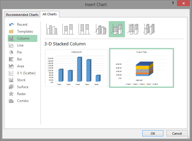 Then, we will position on the Insert ribbon, click on Recommended Charts. In the opened window, first click you should on the All Charts tab, and then select the 3D Stacked Column chart. We choose a 3D column chart, where all values within the series are contained in a single column. This will be the basis for creating a Sales funnel report. Below, we will perform a column transformation. First click on the data column, and then in the newly appeared Format ribbon choose Shape Effects/3-D Rotation, then 3-D Rotation Options. On the right side of the screen, a panel will be opened in which will be offered to transform the column into a pyramid, a partial pyramid, a cylinder, a cone, partial cone… We should select partial Full Cone. By changing the value of Gap Depth and Gap Width we will shape the layout of the graph.

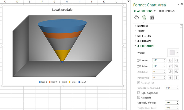
Since the Sales funnel chart is an inverted cone, we will use one trick. The coefficient in cell B1 will be changed to -1. Since this coefficient multiplies all estimated sales values, they will become negative after this procedure, and we get a graphic representation of the inverted cone. Next, we’ll right-click on the cone and select the 3D Rotation option from the context menu. On the right side of the screen, a panel with options for rotating the chart through the axes and forming its display will open. Next, everything is on you. By changing the background style, 3D chart and chart walls, deleting the axes, titles, and further adjusting according to the desired look preferences, we arrive at the final display of the Sales funnel. Like any chart, theSsales funnel interacts in line with the change in the data in the source table. Because of this feature we can use it as a chart for dashboards.