
Searching the ranges
The search of data ranges is most often done with the help of LOOKUP functions, where we enter the criteria value, the search range (table) and the column containing the result values. After entering the formula, Excel finds and displays the requested value. There are several more ways to search the ranges when it is done relative to their position, which will be discussed more in the text that follows …
When we know the position value of the results relative to the value of the search criteria, we use the OFFSET function, whose syntax is:
OFFSET (<range>,<row>,<column>,<height>,<width>)
To understand how this function works, we need to explain what its arguments represent. First one is the address of the cell or the range of cells where we’re performing the search. The row and column are positive or negative values that indicate the X-Y position relative to the search area. If it is a cell, it is a position in relation to a given cell. If it is a range of cells, it is a position in relation to the upper left cell range. Height and width are the number of rows and columns that we want to return as a result. If we want to show the content of a single cell, it will be number 1 (repeated twice). If the OFFSET function is an argument of another function, for example, SUM function, it makes sense to specify multiple cells for height and width. In this way we perform the specification of the range that we want to summarize. Let’s look at some examples:
=OFFSET(C3,-1,-1,1,1)
is the formula by which we show the value of cell B2 (row up, column left, relative to cell C3, one cell x one cell). If we argue that the scope of the formulas would look like this:
=OFFSET(C3:D4,-1,-1,1,1)
This formula also returns the cell B2 value. What would we like to pick up the first three cells in the given table? The formula would look like this:
=SUM(OFFSET(B2,0,0,3,1))

In addition to the OFFSET function, we can use another useful area search function: the INDEX function. Unlike the OFFSET function, where we perform a search in relation to the specified parameters of the specified area, the INDEX function is much more specific. It serves to restore the value of a cell located on the intersection of the desired row and column. There are two forms of this function, and they differ in that they are first used for the bands, and the other for the designated ranges. Their syntax:
INDEX (<range>,<row>,<column>)
INDEX (<range>,<row>,<column>,<range number>)
Let’s show the first method of application. It works by defining the field, and then listing the row and the column in which we want the result to be drawn. For example, if we enter the formula:
=INDEX(B2:D4,2,2)
The desired result is the content of cell C3 (second row, second column, relative to the beginning of the cell, which is B2).
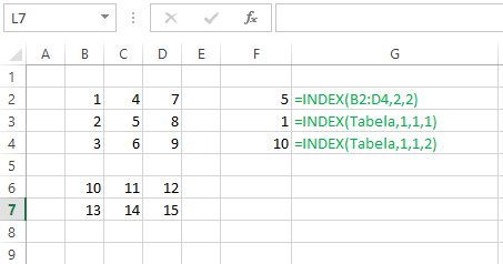
Sometimes we will search for named ranges. They can be unique, but they can also consist of several separate areas. Imagine that we have a named range called the Table, and it consists of areas B2: D4 and B6: D7. In this case, by specifying the regular number of areas, we search in the first or second part of the area. For example, the formula:
=INDEX(Tabela,1,1,1)
shows the content of the cell in the first row and the first column of the first part of the area Tabela. For example:
=INDEX(Tabela,1,1,2)
shows the contents of the cell in the first row and the first column of the second part of this area.
When will we use these functions? Their purpose is primarily to search for unstructured tables. If we want to search structured tables or traditional tables used to store data, it may be better to apply some of the LOOKUP functions.
The MATCH function is used to determine the position of some value in the given array (range) relative to the set criteria, which may be “less than”, “equal” or “greater than”. The syntax of this function is:
MATCH(<search value>,<range>,<criteria>)
For example:
=MATCH(2;B2:B4;0)
would return the value of 2, since the given value (number 2) is placed in the second position in the search string.
Finally, we also mention the function INDIRECT which returns the value of a cell based on its address that is assigned as a text (string). The syntax of this function is:
INDIRECT (<address as a text>, [<parameter>])
The first argument of the function is the address of the cell, given as text. For example, “B2”. If we write the formula:
=INDIRECT(“B2”)
As a result in the cell we get number 1, which is the value that is stored in cell B2. The second parameter, which can be omitted, is TRUE or FALSE. TRUE indicates that the cells are addressed in the “A1” format (the letter as a column mark, the number as a row mark), and FALSE is addressed in the “R1C1” format (and the rows and columns are highlighted in rows).