Forecast of future trends
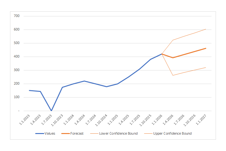
To forecast future trends, you can use the Excel Forecast Sheet option – it’s the fastest and easiest way to see what’s going to happen in the future based on historical data. It uses the FORECAST.ETS function which, in addition to calculating the trend, can also fill in the missing data or recognize the seasonality of the data, and it also uses the FORECAST.ETS.CONFINT function to calculate the confidence interval. How to make a forecast manually?
To calculate and display a trendline in Excel, regression analysis is used. Depending on which mathematical function is chosen, it can be: linear regression, exponential regression, logarithmic, polynomial, power function regression, or moving average method (it’s not regression). You can also predict future trends by using simple Trendline feature. In the specific example, we chose a 6th degree polynomial to calculate the trend line and then, in the Forecast option, we set a rule for Excel to display a forecast for two periods in advance. What the period will be depends on the unit displayed on the x-axis. If the x axis shows months, it will be months. If the years are shown, respectively, it will be years… In some situations, a Trendline can be the solution, but when there is seasonality, missing data, or simply not enough data, it is better to calculate the trends manually.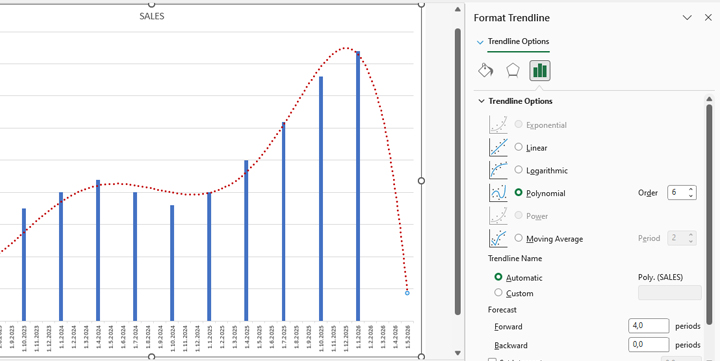
As an example, for manual calculation, we will use a simple table that shows the sales values over time. It contains four columns: YEAR, QUARTER, DATE, and SALES. Although we have defined years and quarters, to make a forecast we need a column that contains dates – hence the DATE column, where we have displayed the date that marks the beginning of the new quarter and the end of the previous quarter. In the SALES column, some arbitrary sales values are given, e.g., sales in millions of euros.
To calculate the trend with the help of linear regression, we can use the TREND function. Syntax:
TREND (<known_y >,<known_x>,<new_x>,<b>)
Arguments:
- known_y – known historical values, e.g. sales value
- known_x – historical independent values, e.g. dates
- new_x – the future value to be calculated.
- b – the default value is TRUE, and if we omit it, the trend is calculated normally. If it is FALSE, it means that the trend line must pass through the zero point (x=0, y=0).
A linear regression function can also be used. Syntax:
FORECAST. LINEAR (<known_y >,<known_x>,<new_x>)
It returns the same values and has a simpler syntax. So if we enter the formula:
=FORECAST. LINEAR (C15,$D$2:$D$14,$C$2:$C$14)
Excel will forecast sales values in the future for the first future quarter. By copying the formula, we get the sales values for all three future quarters.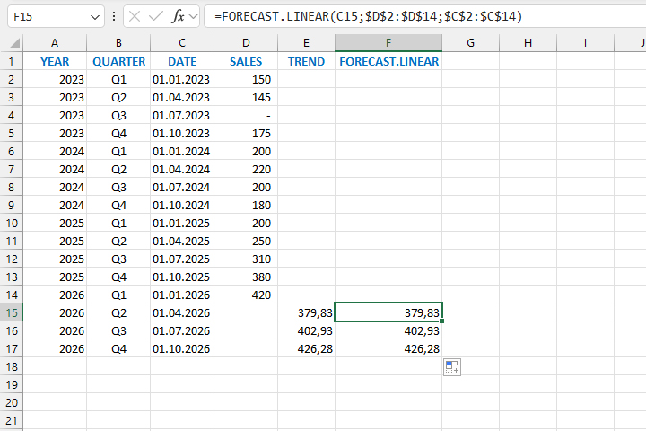
In the previous case, for 2023-Q3, no sales values were shown. If there really wasn’t a sale, that’s not disputed, but what if it’s non-existent data? In this case, we need to perform interpolation to calculate the missing values. The interpolation is calculated using the formula:
=D3+(D5-D3)*(C4-C3)/(C5-C3)
When we fill in the missing values, the TREND and FORECAST.LINEAR will return different results.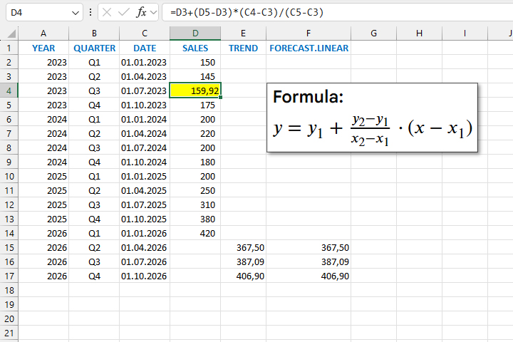
However, to calculate future trends it is best to use FORECAST.ETS function. It predicts future values based on historical data using the Exponential Triple Smoothing (ETS) algorithm, and it can also take into account seasonality, fill in missing data, or perform value averaging for the same date values. Syntax:
FORECAST. ETS (<target_date >,<values>, <timeline>,
[<seasonality>], [<missing_data>], [<aggregation>])
Arguments to the function:
- target_date – the date for which the new value is calculated
- calues – a range (column) with sales values
- timeline – a range (column) with dates
- seasonality – indicates seasonal changes. For example, if you enter a value of 4, it is a signal that changes occur within 4 quarters.
- Missing_data – indicates whether the missing data needs to be filled with interpolation. If the value is 1, interpolation will be performed, and if it is 0, then there has been no sale (the data is 0).
- aggregation– fexample, if you have two equal date values, you can choose which function you want to use to aggregate treir sales data. Most of the time, it’s an average function (1) but you can use some other functions as well.
By entering the formula:
=FORECAST. ETS (C14,$D$2:$D$14,$C$2:$C$14,4,1,1)
we will perform the calculation of future trend values, the function will take into account seasonality (4 quarters), fill in the missing data (interpolation) and perform aggregation for existing dates (AVERAGE).
The upper and lower confidence intervals can be calculated using the FORECAST.ETS.CONFINT function. Let’s enter the formula:
=FORECAST. ETS.CONFINT(C14,$D$2:$D$13,$C$2:$C$13,0.95,1,1)
Now, if you subtract this value from the forecast value, you get the lower confidence interval, and if you add it to the forecast value, the upper confidence interval is calculated.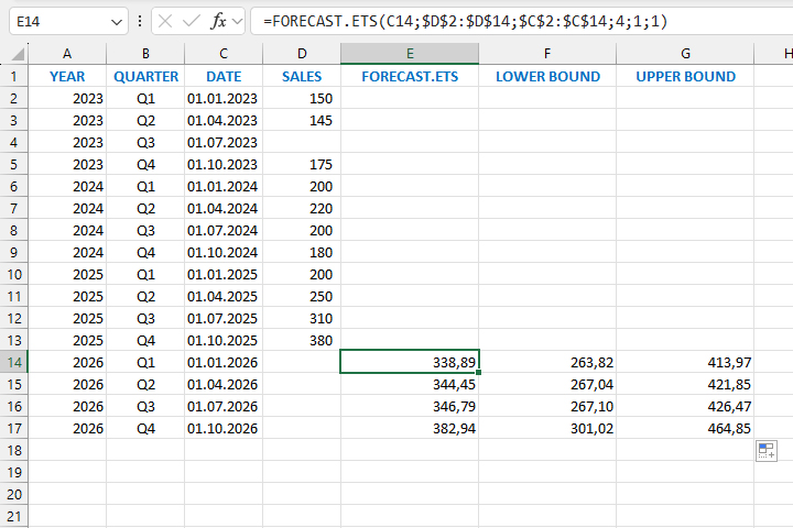
The functions and methods that you have just seen can be used to easily calculate future trends, but if you do not have much experience in these things, it is better to use the Excel Forecast Sheet option.