
Finance tables
How much will our money be worth in the future? Calculating the future and present value of the cash flow is a complex mathematical process. Today it’s easy, because Excel has a class of functions that only deal with this area. Sometimes, in order to facilitate the assessment of the justification of the investment, the so-called “Financial tables” containing discount rates were used to calculate values for the given interest rates and time periods.
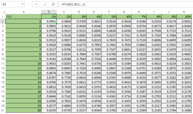
The most commonly used is “Financial Table 2” and it represents the present value of the investment on the assumption that for a certain number of periods, for a given interest rate, we will earn 1 monetary unit. This table is made by creating an Excel spreadsheet where the number of periods (years) is in rows, and columns contain the value of the interest rate. We calculate the discount rate by using the PV function, and to perform this should enter the formula in the first cell of the table (B2):
=PV(B$2,$A3,,-1)
In order to properly copy the formula it is necessary to fix the second row in the first argument of the function, as well as the first column representing its second argument. Now we need to copy the formula into the remaining cells and further format the values as decimal numbers with 4 decimal places.
Financial table no. 2 is used when we have different net cash flow values. When they are the same we will use the Financial Table no. 1 containing cumulative discount rates. We create it by copying the previous table into a new worksheet. The first row of the table retains the formula as in the previous example. In the first cell of the second row (B3) should enter the formula:
=PV(B$1,$A3,,-1)+B2
By copying this formula into the remaining cells in the table we have created the Financial Table no. 1.
