Randomly generated data

What is the most common problem for programmers and report makers? Certainly, it is a lack of adequate information they need to launch the report and see if it works. Data can be entered manually. But hey: imagine yourself to manually enter 100,000 records!?! This article demonstrates simple techniques to create tables with data to test the most demanding reports.

In the example that follows we’ll create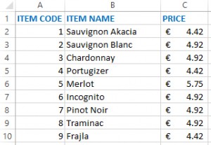 a pivot table to analyze sales data for 100,000 entries representing the sales transaction occurred during the period from 1st January to 31st December of 2015. Transactions will be randomly generated on the basis of the table with the items. Item names and prices are taken from a web site of famous Serbian winery „Mačkov podrum“ (that has a good web site and even better wines). Table of Items, stored in homonymous worksheet, consists of ID, ITEM NAME and PRICE and it is populated with data about wines. The main table (Transactions) will be part of worksheet named Transactions. Here we’ll randomly generate the sales data.

First, let’s create a header of the Transactions table with: S/N, ITEM CODE, ITEM NAME, QUANTITY, PRICE and AMOUNT. Then we need to generate serial numbers. Go to the cell A2 and enter the value 1. Then select all cells in the same column by pressing CTRL+SHIFT+arrow down key. Next you should go to the Home ribbon and select option Series from Fill menu. A dialog box will appear. Enter the value of 100,000 in a box named Stop value, and then press OK. The table will be populated with serial numbers that go from 1 to 100,000.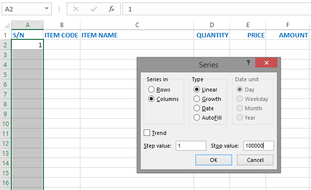

Now we need to randomly generate items. Select cell B2 and enter the formula:

=RANDBETWEEN(1,9)

It will randomly select an item code. Cell B2 is surrounded by a box, with a small square in down right corner. If we double click it the formula will be automatically copied throughout the column, from first to last row.

Next we’ll go to the cell D2 to enter the formula that generate quantities. To do that we’ll multiply a random number between 1 and 10 with number 6 (since one box of wine contains 6 bottles). Enter the formula:

=RANDBETWEEN(1,10)*6

and then repeat the process of copying values throughout the column.

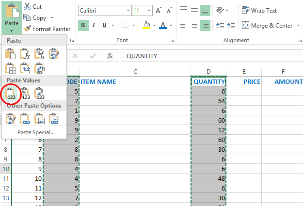
Random values have one flaw. Each time we recalculate the spreadsheet their value will change. To avoid that we need to select values in columns B and D. Click F5 to open GoTo dialog box, and then in the Reference field enter „B:B“. Then click CTRL+C to copy the values to Clipboard, and after open the Paste menu in Home ribbon and select Paste Values option. Repeat the procedure for column D, and all random numbers will be converted to numeric values.

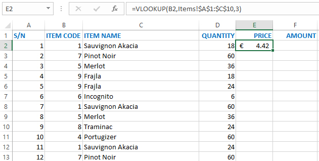
Now we have to populate columns ITEM NAME and PRICE. We’ll do that by using VLOOKUP function that will help us to find appropriate values in the Items table. Click to C2 and enter the formula:

=VLOOKUP(B2,Items!$A$1:$C$10,2)

Later, copy the formula throughout the column. Click on E2 and enter the formula:

=VLOOKUP(B2,Items!$A$1:$C$10,3)

and copy the formula throughout the column. You may also change the format. To do that first press CTRL+SHIFT+1. Then, go to the „dollar mark menu“ in Home ribbon and choose the option that will show prices in euros.

The last step we have to do is calculating the amount. Go to cell F2 and enter the formula:

=D2*E2

As you guess, now you only need to copy the formula to fill remaining values in the column. Now we have randomly generated table that can be used further for creating all kinds of reports.