Customizing source table

Before you decide to create a pivot table, ask yourself: do you really need it? This report groups and aggregates data (summation, averaging, counting, etc.) and you may have already done so in the source table; maybe it is, in itself, a report? If you do decide to take this step, you will need to adjust it so that the pivot table can process the data, because it requires that the records be in rows.

As an example, we will start from the table which contains data on the success of students in primary schools. The first two columns represent the name of the school and the student. The following are the columns with the number of grades (1-5) that the student received during the year. The table shows the grades over a period of three years. As you can see, the source table is a report. In order for the pivot table to be able to work with this data, it is necessary to transform them, i.e. it is necessary to rotate the columns with the number of achieved grades. Theoretically, we could do this with the help of the TRANSPOSE function and a lot of hard work. Fortunately, Power Query offers us a much more elegant solution.

First, create a Data Table from the source and then import it into the Power Query Editor. Select only the columns that contain the grades. Then, in the Transform ribbon, select the Unpivot Columns option.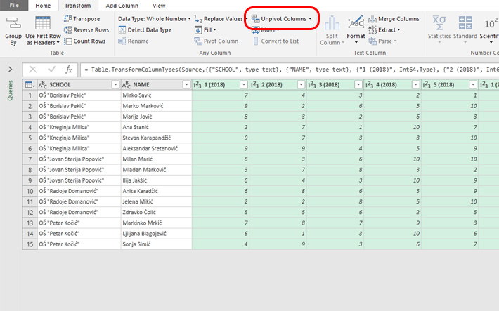

Power Query will perform rotation and as a result you have two new columns: Attribute and Value. The first contains grades and years, and the second contains the number of grades achieved.

The Attributes column should first be divided into two, the first of which will contain the name of the grade (1-5) and the second the year. First select Split Column and then split by using the By Delimiter option. Let the separator be Space, and you select the first left character.

The result is two columns. You can immediately rename the first header to GRADE. The second column became a negative number after the transformation. To get the year, go to Transform ribbon, then to Scientific menu and choose option Absolute Value. Rename the header of this column to YEAR. Rename the header of the third column to NUMBER. After selecting the Close&Load option, you will get a source suitable for creating a pivot table.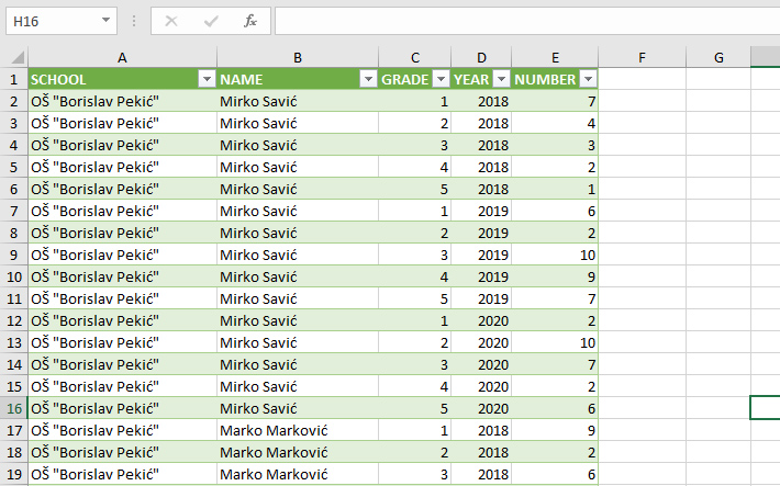

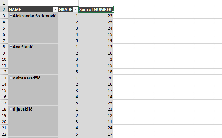
Finally, let’s make a pivot table! Click somewhere inside the source table, then select the Pivot Table option in the Insert ribbon and create pivot table report in a new worksheet. We will add the dimensions NAME and GRADE in the Rows field, and the NUMBER in the Values ​​field. As a Report Layout we can choose the Tabular Form, hide subtotals, change the style of the table. And voila!