Filtering by lists

Slicers are great feature, but unfortunately they can not be used to filter traditional Excel reports. If we use the conditional aggregation functions, in order to calculate the desired values, as well as the data validation technique, we can make simple but effective filters by selecting the values from the list. By selecting the criteria from the list, the automatic update of the values in the report is performed. Let’s see how this works!

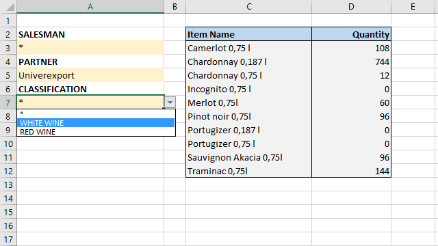
In order to be able to create a report, a table is required containing business transaction data. It should contain sales quantites, as well as the reporting dimensions that we want to use as filters. To begin with, in a separate worksheet we will add each of the desired dimensions by copying the column, then by removing duplicates in order to get unique values. The first of the values should be asterisk.

Then, in a similar way, we will add item labels to the worksheet where the report will be located. On the left, in the first column, we will envision several fields that will be used as filters. Using the data validation technique, should set the values in the „cell-filters“ to be selected from the list that is created based on the values of the reporting dimensions that we have previously added.

Finally, by using the SUMIFS function, we need to create a formula which calculates quantities sold based on the product name and given cell-filter values:

=SUMIFS(TT[QTY];TT[ITEM];C3;TT[SALESMAN];$A$3;TT[PARTNER];$A$5;
TT[CLASSIFICATION];$A$7)

Cell-filter addresses should be fixed. After we create the formula, it is still necessary to copy it into the remaining cells and to beautify the report.