Testing a condition – Excel kitchenette

Testing of the conditions is done so that, depending on its fulfillment, we will get different results. These can be some concrete values, but most often, depending on the fulfillment of conditions, we devise different formulas for calculating. It is possible to create multiple conditions (multi-branching) or as a condition to specify an index that determines which expression will be calculated. The following text will detail the logical functions for testing the conditions.

The most commonly used condition test function is IF. It has three arguments: logical condition, value if true and value if false. Its syntax is:

IF (<logical test>,<value if TRUE>,<value if FALSE>)

Condition represents a logical test, and result (true/false) could be a value, name, cell adress, formula… For instance, if we want to if we want to check if 2> 1, and if it is that the cell value becomes “YES”, and if it does not become “NO”, we will write the following formula:

=IF(2>1,”YES”,”NO”)

As a result we’ll have a cell that shows “YES”.

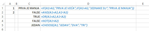
As a result we can use an expression or even another IF function. For instance, let’s write a formula that compares values of two cells. If the first is bigger than another result is “FIRST IS BIGGER”. If they are equal result should be “THEY ARE EQUAL”, and otherwise “FIRST IS SMALLER”:

=IF(A1>A2,”FIRST IS BIGGER”,IF(A1=A2,”THEY ARE EQUAL”,”FIRST IS SMALLER”))

When entering formula in Excel, it automatically paints parentheses in different colors to make it easier for us to see where a certain function ends. The most common mistake that occurs when entering such formulas is to omit the brackets, so pay attention to it.

In addition to the IF function, the AND, OR, XOR, and NOT functions are also used to test conditions. They compare one or more conditions. The AND function, if all conditions are met, returns TRUE; otherwise it returns the value FALSE. The OR function has the same syntax, but to return the correct value requires at least one of the conditions to be met. The XOR function is an “exclusive OR” and returns TRUE only when one of the conditions is true and not both. The NOT function is used to “negate” a condition. That is, if the condition is met, it returns the value FALSE, and if it is not, it returns the value TRUE. The syntaxes of these functions are:

AND (<logical test₁>,<logical test₂>,…,<logical test_n>)

OR (<logical test₁>,<logical test₂>,…,<logical test_n>)

XOR (<logical test₁>,<logical test₂>,…,<logical test_n>)

NOT (<logical test>)

The last function that we have here is the CHOOSE function. It is used for multiple branching, ie for choosing one of the many results depending on the value of the index. The index is the integer number that indicates the ordinal number of the starting point. Syntax:

CHOOSE (<index>,<result₁><result₂>,…,<result_n>)

For example, if, depending on the cell A1 value, we want to get the name of a number, we will write the formula:

=CHOOSE(A1,”ONE”,”TWO”,”THREE”)

In the case that A1 has a value of 1, 2 or 3 in the cell, the name of that number will be displayed. When working with this function, it is only important to perform a data validation in the cell, ie to allow only the input of those indexes for which the function can return the starting value. Otherwise, there will be errors.