
Refilling shelves
I often get upset when I go to the supermarket and see the workers closing the passages by racking up the shelves. How to help them? If a company has implemented an ERP, it is possible to extract a stock report, critical inventory, and a place where the items are located (warehouse, location, position). With a little imagination and knowledge of conditional formatting techniques, there is an easy way to mark those shelves and positions where urgent refill is required.
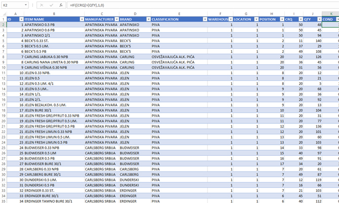
To begin with, you need to use an existing ERP report or write a query that generates a table with the necessary data. We will assign the name to the table, e.g. “Supplies”. It should include general information about the item: code, name, manufacturer, brand, classification … It should also contain the label of the warehouse, location and position, as well as the stock level and critical stock level. In order to create a report, it is necessary to manually add another column where should enter the formula:
=IF([CQT]>[QTY],1,0)
In this formula we compare stock levels with critical stock levels. If the first level i smaller then second it means that item should be refilled.
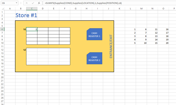
Now the creative part follows. We will draw in Excel a map of a store with shelves, cash registers and other related objects. In this particular case, we use only two shelves, each with 20 positions. In practice, this would be a lot more because in average supermarket there are always a few thousands of items.
In fields that indicate positions (shelves) should write a formula that summarizes all those items that need to be urgently refilled for the given location and position. To make it easier to write a formula to the right, a temporary table with position labels (1-20) is added, which we can hide later. In the first cell of the table we enter the formula:
=SUMIFS(Supplies[COND],Supplies[LOCATION],1,Supplies[POSITION],L6)
If you did it all right you’ll get the number of items that should been refilled promptly.
Further, copy the formula into remaining cells. Then, we’ll repeat the process for another shelf:
=SUMIFS(Supplies[COND],Supplies[LOCATION],2,Supplies[POSITION],L6)
We also fill in all the remaining cells, and then hide the temporary table on the right.
When we get tables with the number of items to be refilled we still need to apply the conditional formatting technique. In the Home Ribbon, open the Conditional Formatting menu, and then select Highlight Cell Rules / Greater Than and mark that the rule applies to all those cells whose values are greater than zero. Repeat the procedure in both tables (for both shelves). Positions that should be refilled are clearly highlighted.
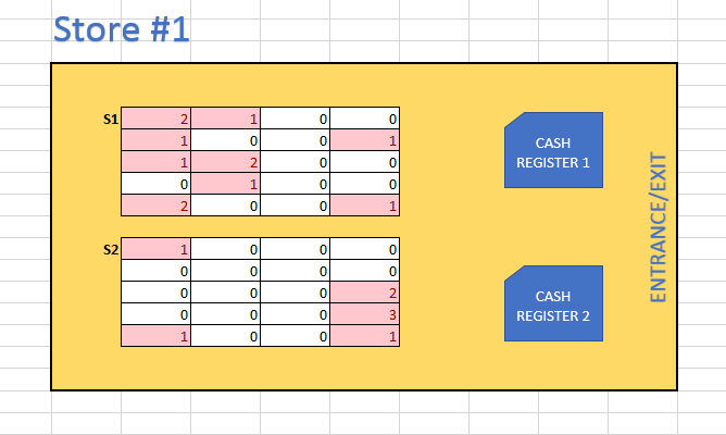
As you can see this is a very simple technique and it can be used to get a variety of useful reports: which items are missing on the shelf, whether there are items that expire, whether a manufacturer or a brand is not positioned well enough… The possibilities are infinite, it all depends on the creativity of analysts of business reporting. Hooray for Excel!