Advanced data grouping

In one of the previous “recipes” we talked about how to use the Excel GROUPBY function. On that occasion, you could find out how to use it in one of the standard scenarios of its application, and now you will learn how to use it in a slightly more advanced way. To begin with, how you can group by two or more dimensions, and then how to display percentages, determine the depth of the calculation, and so on.

Let’s start, like last time, with an example where we have a structured table (ST) that shows sales transactions in a certain period of time. The standard way to use the GROUPBY function would be to perform grouping and aggregation based on one of the columns. For example, by creating the formula:

=GROUPBY(TR[CLASSIFICATION],TR[AMOUNT], SUM)

The result is a simple table that shows the total sales in relation to the classification.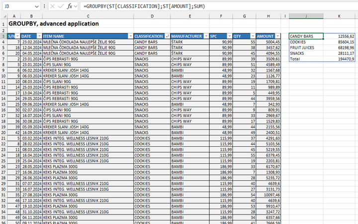

How do we group data by multiple columns? The GROUPBY function, where we specify the columns to be grouped, accepts only one argument, so we will use a simple trick; That is, we will use the HSTACK function, which groups multiple given ranges next to each other. For example, the formula:

=HSTACK(ST[CLASSIFICATION],ST[ITEM NAME])

Creates a dynamic table that displays all the elements of the CLASSIFICATION and ITEM NAME columns by each other. If we add it as the first argument to the GROUPBY function:

=GROUPBY(HSTACK(ST[CLASSIFICATION],ST[ITEM NAME]),ST[AMOUNT], SUM)

The result is a table in which the grouping is first done by classification, and then by the name of the item, while the last column shows the total sales, i.e. the sum of all values in the AMOUNT column.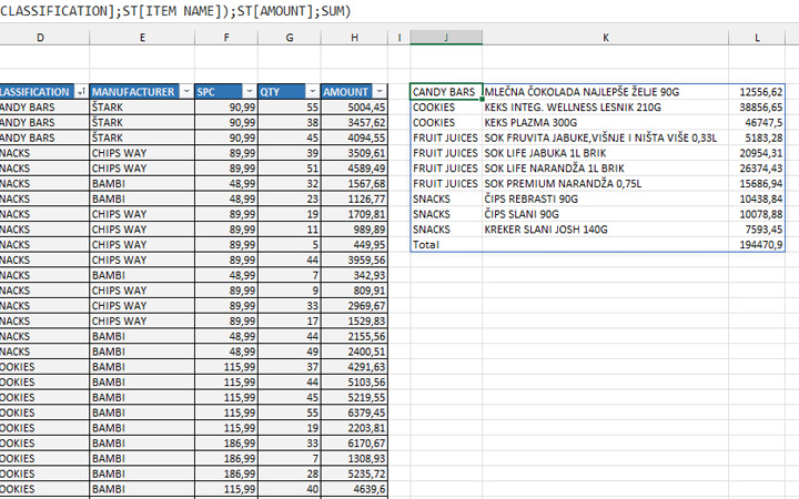

What if we wanted to calculate the total value of the quantity and amount? No problem, we’ll use HSTACK in place of the second argument:

=GROUPBY(HSTACK(ST[CLASSIFICATION],ST[ITEM NAME]),HSTACK(ST[QTY],ST[AMOUNT]); SUM)

As a result, we will get the following table: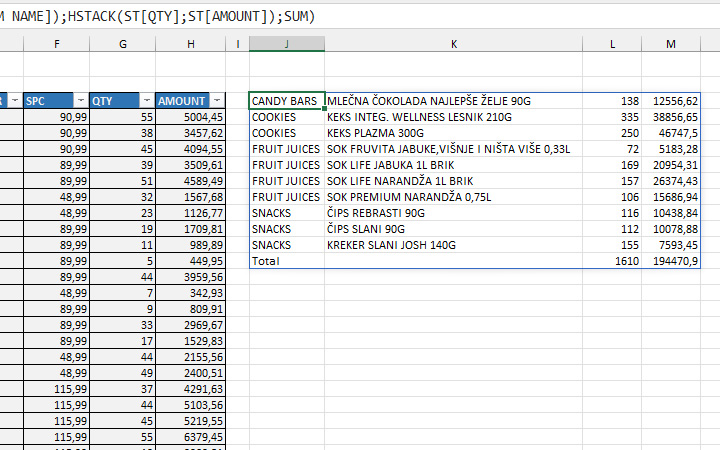

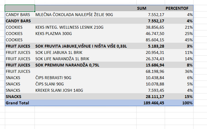
What if we wanted to group by classification and item name, but with the display of group headers, subtotals, and grand totals? Let’s create a formula:

=GROUPBY(HSTACK(ST[CLASSIFICATION],
ST[ITEM NAME]);ST[AMOUNT], HSTACK(SUM; PERCENT), 3, 2)

If we format the table a bit more we will get a very nice, dynamic report.