Formatting dynamic results
Since 2018, Excel has undergone one of the biggest transformations in its history with the introduction of functions for working with dynamic arrays. Unlike traditional functions that return a single value, these functions can generate entire tables as a result. Because these tables are dynamic, any change to the data in the source is automatically reflected in the displayed result. How to format dynamic results?
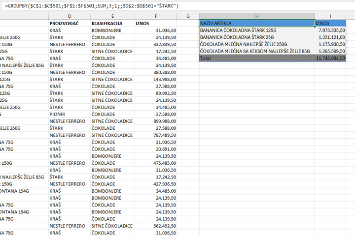
In the picture you can see the range of data in which the data on the sale of chocolate products are located. With the help of the dynamic GROUPBY function, we extracted the data into a report that shows sales in relation to the name of the item.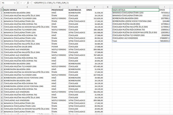
The range where the formula returned the result does not have any formatting. If we just want to format the sales values, it is enough to select the column and apply the shortcut CTRL+1, which converts the numbers that are automatically displayed using the General format to Decimal, with two decimal places. The rest of the table will be dynamically formatted by applying a few conditional formatting rules.
The last line contains the word “Total”. If we want to put a gray background on the last line, we’ll create a new conditional formatting rule using the formula:
=$H1=”Total”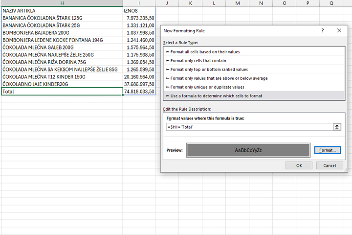
After entering the formula, we set the dark gray background color, and by clicking OK we will confirm the rule.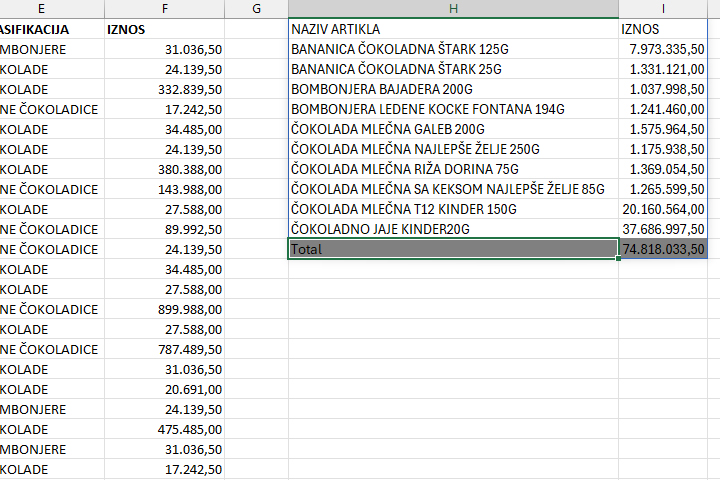
If we want to color all the rows in the table light gray, we will add the rule:
=IF(AND($H 1<>””; ODD(ROW())); TRUE; FALSE)
However, since the rule for “Total” is after the newly added rule, we need to move it one position above and give it priority.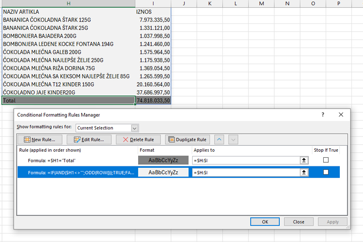
Finally, we will add another rule that colors the table header background in blue.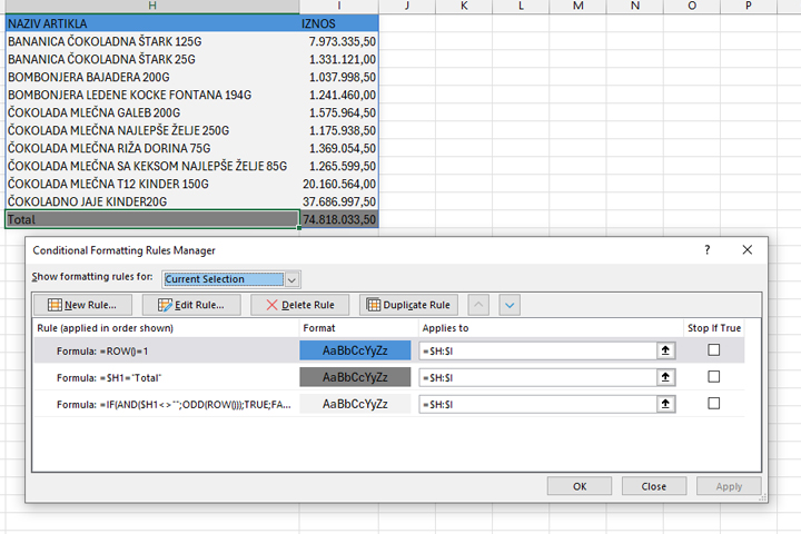
When we apply conditional formatting to specify the display of dynamic tables, if the formula changes or there is a change in the data source the table will retain previously defined formatting…