
Lists as function arguments
Excel has recently made it easier to work with formulas that use arrays and constants – you no longer have to save them by pressing CTRL+SHIFT+ENTER! We can now use lists of values, given in curly brackets, as function arguments. This is great news, and the possibilities are manifold. In the following post, you will be able to see the real application of this feature…
Let’s start from the beginning. If you want to display a dynamic list consisting of numbers 1, 2 and 3, you can write the following formula:
={1; 2; 3}
The result is the values 1, 2 and 3 displayed in the column. If you were to write a formula:
={1\2\3}
Excel would create a dynamic list in a row that displays the values 1, 2, and 3 in a row.
Imagine if you had to list the dates with which the first three months of 2026 begin? Let’s write the formula:
=DATE(2026;{ 1; 2; 3}; 1)
The start dates of the first three months of 2026 will also appear in the column.
Perhaps the best application of this feature is within the VLOOKUP function. Imagine a scenario in which you need to find the values of several columns from the Items table and show them in the Transactions table. Let’s write the formula:
=VLOOKUP(F2,$A$2:$C$6,{ 2\3}; FALSE)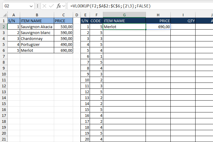
Creating master data table has never been easier, right? As an argument for separating lists, we use “,” and “;” for English region settings, and “;” and “\” for “Serbian Latin” for Serbian and some other region settings.