The Top N items

If you want to single out those with the highest or lowest price from the list of items, the simplest way is to turn on the Autofilter option, and then apply the Top 10 numerical filter over the column where prices are stored. There is another, equally accessible way – with the aid of the LARGE and SMALL functions, which you can use to identify the ranking of an item based on the sale price. Add to this dynamic filters and the process will be even simpler.

To see how this works, we’ll start with a simple example. The table holds the data about the items: name, sales group, classification, supplier, manufacturer, brand, purchase price, selling price and quantity in stock.

Using the formula:

=LARGE(Artikli[PC],{1,2,3,4,5})

Excel extracts the five items with the highest selling price from the PC column in the Items table (Top 5). Notice the notation in the second argument, which is used to specify the rank. When you add multiple values of constants in curly brackets, you are instructing Excel to form a dynamic array and use each of the specified values in turn in the formula.

Suppose the sales prices are unique. In this case, using the XLOOKUP function and the “#” sign, which indicates that you take the dynamic values from the formula, we can write the following expression:

=XLOOKUP(M2#, Article[PC], Article[NAZIV ARTIKLA],””)

This formula returns the name of the item in relation to the previously extracted prices.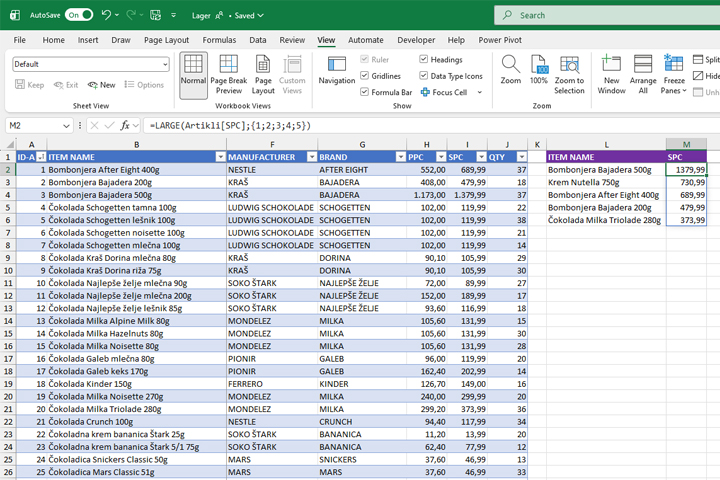

This is the criterion for extracting the five highest prices (Top 5). If we had used the SMALL function instead of the LARGE function, we would have been able to extract the five lowest prices (Bottom 5) in a separate table in the same way.